CIGVis - a tool for visualizing multidimensional geophysical data#
Overview#
cigvis is a tool for visualizing multidimensional geophysical data, developed by the Computational Interpretation Group (CIG). Users can quickly visualize data with just a few lines of code.
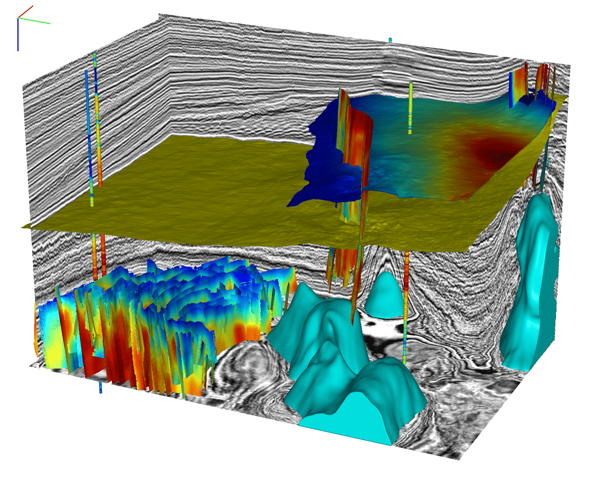
cigvis can be used for various geophysical data visualizations, including 3D seismic data, overlays of seismic data with other information like labels, faults, RGT, horizon surfaces, well log trajectories, and well log curves, 3D geological bodies, 2D data, and 1D data, among others. Its GitHub repository can be found at github.com/JintaoLee-Roger/cigvis, and documentation is available at https://cigvis.readthedocs.io/.
cigvis leverages the power of underlying libraries such as vispy for 3D visualization, matplotlib for 2D and 1D visualization, plotly for Jupyter environments (work in progress), and viser for web-based visualization (SSH-Friendly). The 3D visualization component is heavily based on the code from yunzhishi/seismic-canvas and has been further developed upon this foundation.
CIGVis: An open-source Python tool for the real-time interactive visualization of multidimensional geophysical data Jintao Li, Yunzhi Shi, Xinming Wu Paper: https://library.seg.org/doi/abs/10.1190/geo2024-0041.1
Installation#
To install via PyPI, use
# only with vispy and PySide6, for desktop
pip install "cigvis[gui]"

# only with plotly, for jupyter
pip install "cigvis[plotly]"

# only with viser, visualizing in browser
pip install "cigvis[viser]"

# only with Panel + Plotly, for SSH-friendly 2D slice viewing
pip install "cigvis[sliceviewer]"

# install all dependencies
pip install "cigvis[all]"
For local installation, clone the repository from GitHub and then install it using pip:
git clone https://github.com/JintaoLee-Roger/cigvis.git

# only with vispy and PySide6, for desktop
pip install -e ".[gui]" --config-settings editable_mode=compat

# only with plotly, for jupyter
pip install -e ".[plotly]" --config-settings editable_mode=compat

# only with viser, visualizing in browser
pip install -e ".[viser]" --config-settings editable_mode=compat

# only with Panel + Plotly, for SSH-friendly 2D slice viewing
pip install -e ".[sliceviewer]" --config-settings editable_mode=compat

# install all dependencies
pip install -e ".[all]" --config-settings editable_mode=compat
Core Features#
Convenient 3D geophysical data visualization.
Ongoing development of 2D and 1D data visualization.
Additional colormaps tailored for geophysical data.
Rapid display of large data in OpenVDS format.
Usage#
Basic Structure#
The fundamental structure of cigvis’s visualization code consists of:
1. Data loading
2. Creating nodes
3. Passing nodes to the plot3D function
4. Optionally grouping view, save, colorbar, and GUI settings
For example
import numpy as np
import cigvis

# Load data
d = np.fromfile('sx.dat', np.float32).reshape(ni, nt, nx)

# Create nodes
nodes = cigvis.create_slices(d)

# Visualize in 3D
cigvis.plot3D(nodes)
This basic code structure allows you to quickly visualize your geophysical data using cigvis. Simply load your data, create nodes, and pass them to the plot3D function as demonstrated in the example above.
For new code, plot3D options should be grouped by ownership:
cigvis.plot3D(
    nodes,
    view=cigvis.Plot3DView(
        size=(900, 700),
        grid=(1, 2),
        share=True,
        xyz_axis=False,
        azimuth=-65,
        elevation=22,
    ),
    save=cigvis.Plot3DSave(
        path='example.png',
        transparent_bg=True,
    ),
    gui=cigvis.Plot3DGui(enabled=False),
)
view controls the VisPy canvas, layout, and camera; save controls automatic screenshot behavior; cbar controls colorbar export options; and gui controls the optional PySide6 GUI shell. Legacy top-level parameters such as size=, savename=, grid=, share=, xyz_axis=, and cbar_region_ratio= are deprecated since 0.2.1 and scheduled for removal in 0.4.0.
Backend APIs are now explicit. Use top-level cigvis.create_* and cigvis.plot3D for VisPy rendering. In Jupyter notebooks, do not rely on cigvis.create_* to switch to Plotly automatically; import the backend namespace explicitly:
from cigvis import plotlyplot

nodes = plotlyplot.create_slices(d)
# Optional overlays follow the same flow as the VisPy backend:
# nodes = plotlyplot.add_mask(nodes, mask, cmap='jet', interpolation='nearest')
plotlyplot.plot3D(nodes)
Camera and Dragging#
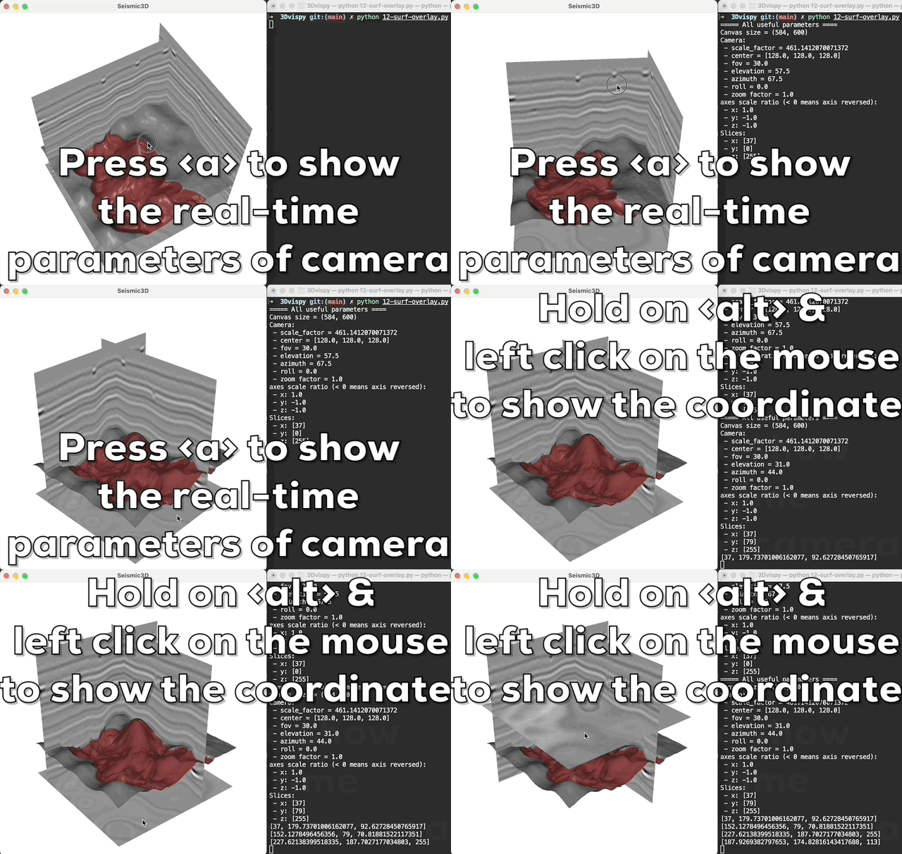
Left click and drag to rotate the camera angle; right click and drag, or scroll mouse wheel, to zoom in and out. Hold <Shift> key, left click and drag to pan move. Press <Space> key to return to the initial view. Press <S> key to save a screenshot PNG file at any time. Press <Esc> key to close the window.
Hold <Ctrl> key, the selectable visual nodes will be highlighted when your mouse hovers over them; left click and drag to move the highlighted visual node. The volume slices will update their contents in real-time during dragging. You can also press <D> key to toggle the dragging mode on/off.
Press <z> to zoom in z axis, press <Z> or <Shift> + <z> to zoom out z axis.
Press <f> to increase fov value, press <F> or <Shift> + <f> to decrease fov value.

Press <s> to save a screen shot.
Press <a> to print the camera’s parameters in real-time; hold on
the <alt> (or <option> in macos) and left click the mouse to
show the coordinate of the click point in the 3D volume.
Various Geophysical data#
In cigvis, we represent various geophysical data as individual nodes, assemble these nodes into a list, and then pass this list to the plot3D function for visualization.
We visualize a three-dimensional data volume as multiple slices along the x, y, and z directions. Additionally, we can overlay other three-dimensional data slices on these slices, allowing users to interactively drag them along an axis using the mouse.
Horizon data can be represented as scatter points with a shape of (N, 3), or as z-values on a regular grid of size (n1, n2).
Well log trajectories are displayed as tubes, where the size of the first well log curve is represented by the color and radius at each position along the tube. Other well log curves are displayed as surfaces attached to the tube’s edge. An example is shown below (code available at cigvis/gallery/3Dvispy/09).
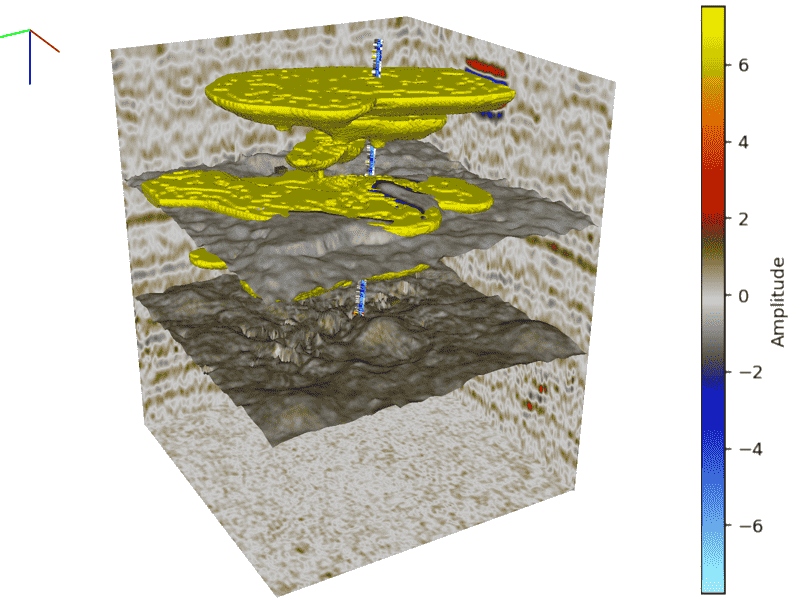
These capabilities within cigvis allow for versatile and interactive visualizations of a wide range of geophysical data types, enhancing the understanding and analysis of such data in geoscience applications.
Multivolumes in One Canvas#
You can pass multiple independent node combinations to the plot3D function and set a grid through view=cigvis.Plot3DView(grid=(2, 2)). This divides the canvas into multiple independent sub-canvases, where each sub-canvas displays a separate 3D data set within the same canvas. The example code for this can be found in the documentation
at cigvis/gallery/3Dvispy/10.
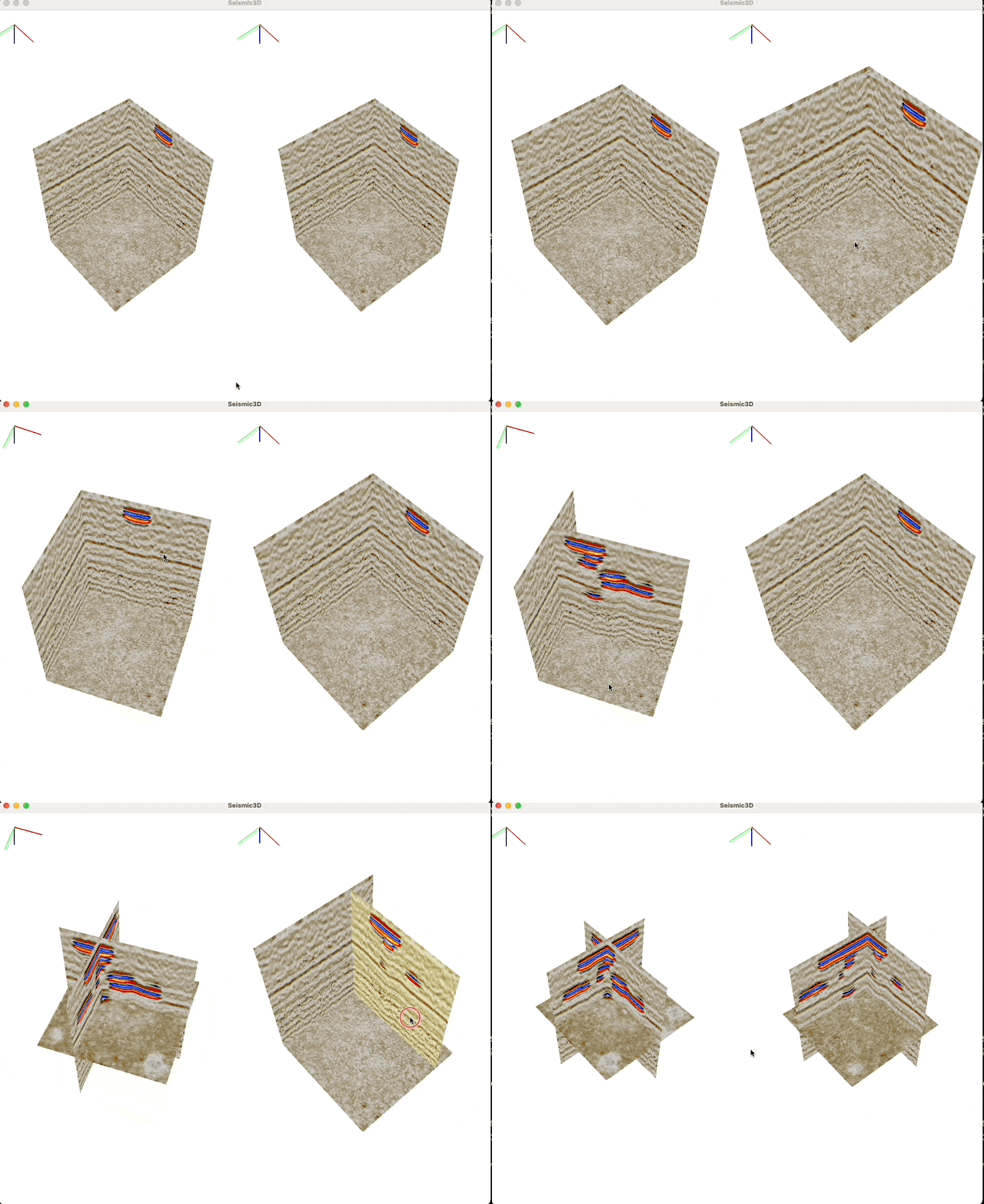
Furthermore, you can link the cameras of all sub-canvases together with view=cigvis.Plot3DView(share=True). This means that any rotation, scaling, or slicing performed in one sub-canvas will be mirrored in all other sub-canvases, ensuring that they all exhibit the same changes simultaneously. This feature is highly advantageous when comparing multiple sets of data, such as results from different experiments, results alongside labels, seismic data compared with attributes, and more.
You can find example code for this functionality in the documentation
at cigvis/gallery/3Dvispy/11.
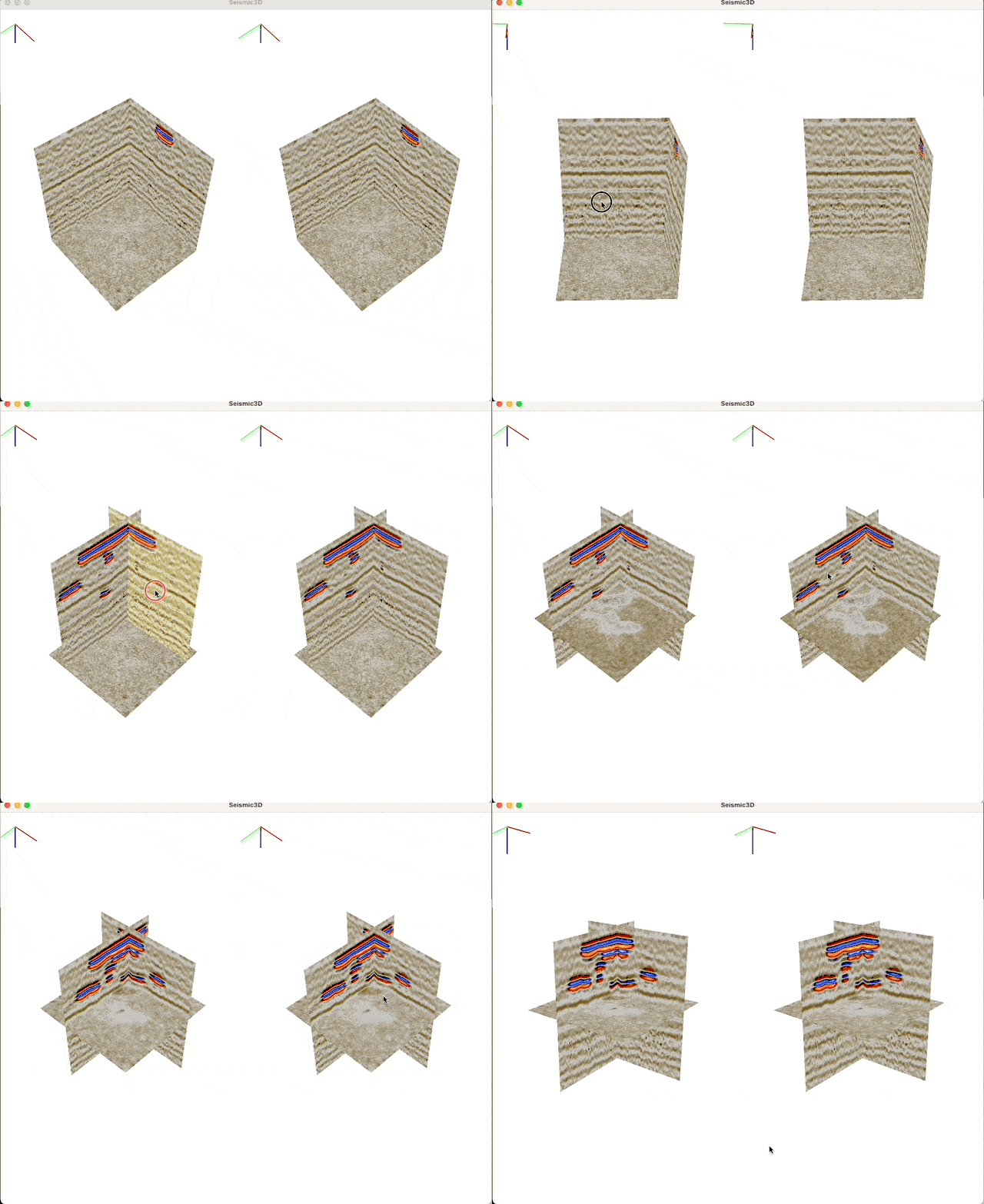
These capabilities provide a powerful way to visualize and compare multiple independent 3D data sets within a single canvas using cigvis.
Web-based Visualization#
Based on viser, cigvis also supports visualization 3D data in web/browser environment with just a few lines changed. All you need to do is simply replace cigvis with viserplot, see follows:
   import numpy as np
   import cigvis
+   from cigvis import viserplot

   # Load data
   d = np.fromfile('sx.dat', np.float32).reshape(ni, nt, nx)

   # Create nodes
-   nodes = cigvis.create_slices(d)
+   nodes = viserplot.create_slices(d)

   # Visualize in 3D
-   cigvis.plot3D(nodes)
+   viserplot.plot3D(nodes)
When you are in a jupyter environment, we recommend maintaining a unique server,
otherwise the port will be changed.
   import numpy as np
   import cigvis
+   from cigvis import viserplot
+   server = viserplot.create_server(8080)

   # Load data
   d = np.fromfile('sx.dat', np.float32).reshape(ni, nt, nx)

   # Create nodes
-   nodes = cigvis.create_slices(d)
+   nodes = viserplot.create_slices(d)

   # Visualize in 3D
-   cigvis.plot3D(nodes)
+   viserplot.plot3D(nodes, server=server)
After calling viserplot.plot3D, it will generate some logs like:
╭─────────────── viser ───────────────╮
│             ╷                       │
│   HTTP      │ http://0.0.0.0:8080   │
│   Websocket │ ws://0.0.0.0:8080     │
│             ╵                       │
╰─────────────────────────────────────╯
If you are running the code on your local machine, just open 0.0.0.0:8080 in your
browser to see the image. If you are running the code on a remote server
(yes, cigvis also works when connected remotely using ssh!),
you can enter {ip}:8080 in the browser to see the
visualization (ip is the ip of remote server, e.g., 222.195.77.88:8080).
It is not possible to divide multiple canvases in the browser, i.e. it is not possible to visualize multiple canvases in a tab, which may cause some trouble when comparing different results. But we can use some tricks to achieve this, see this example (cigvis/gallery/viser/04):
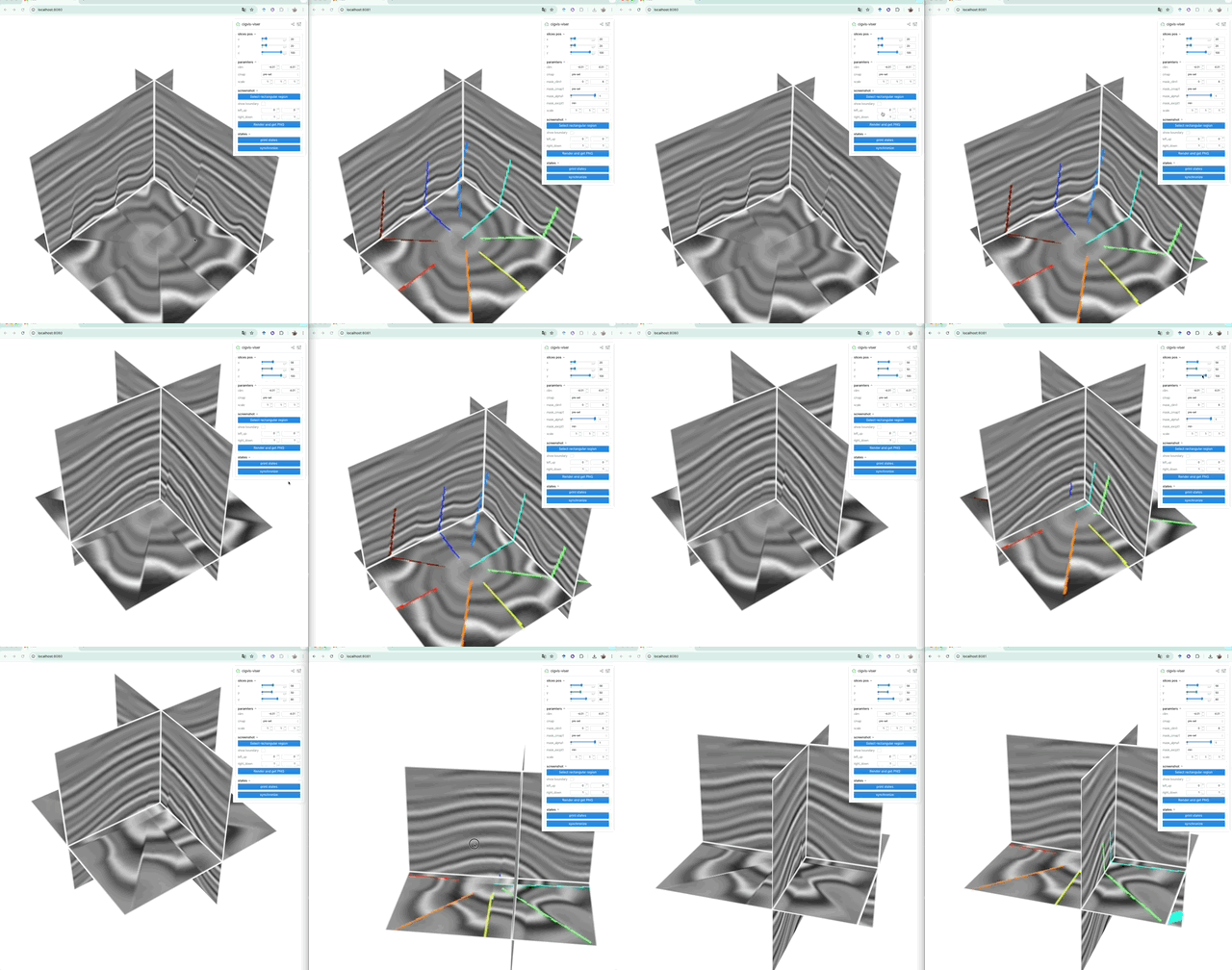
There are several examples in gallery/viser for reference.
SSH-Friendly 2D SliceViewer#
For remote servers where OpenGL is unavailable or a 3D/4D scene is too heavy, cigvis.sliceviewer provides a lightweight browser-based 2D viewer. It renders one chosen 2D plane from a 2D/3D/4D array with NumPy/Plotly and serves it through Panel:
import numpy as np
from cigvis import sliceviewer as sv

volume = np.fromfile('sx.dat', np.float32).reshape(4, ni, nx)
nodes = sv.create_slice(
    volume,
    display_axes=(1, 2),  # rendered as (Y, X)
    indices={0: 2},       # fixed index for hidden dimensions
    aspect=1.0,
    cmap='gray',
    interpolation='nearest',
    render_mode='float',
)

# Forward the port first when running through SSH:
# ssh -L 5007:localhost:5007 user@server
sv.show(nodes, port=5007)
The sidebar can switch Y axis / X axis, swap X/Y, change fixed indices for the hidden dimensions, adjust aspect (equal, free, or a custom Y/X ratio), choose RGBA image vs float heatmap rendering, and choose interpolation (nearest, linear, best, or auto). If display_axes is omitted, the two largest dimensions are displayed automatically.
For before/after comparison, pass two or three node lists and choose a grid:
nodes_raw = sv.create_slice(raw, display_axes=(2, 3), indices={0: 1, 1: 2})
nodes_out = sv.create_slice(processed, display_axes=(2, 3), indices={0: 1, 1: 2})

sv.show([nodes_raw, nodes_out], grid=(1, 2), port=5007)
For more panels, choose any grid large enough for the inputs, for example grid=(2, 2).
For scripts and tests that only need the Panel object, call sv.show(nodes, launch=False) or sv.build_layout(nodes).
sliceviewer binds to localhost by default, which works for local browsing and SSH port forwarding. Use address='0.0.0.0' only when other machines need to connect to the server process directly.
Citations#
If you find this work useful in your research and want to cite it, please consider use this:
Plain Text
Li, J., Shi, Y. and Wu, X., 2024. CIGVis: an open-source python tool for real-time interactive visualization of multidimensional geophysical data. Geophysics, 90(1), pp.1-37.
BibTex
@article{li2024cigvis,
title={CIGVis: an open-source python tool for real-time interactive visualization of multidimensional geophysical data},
author={Li, Jintao and Shi, Yunzhi and Wu, Xinming},
journal={Geophysics},
volume={90},
number={1},
pages={1--37},
year={2024},
publisher={Society of Exploration Geophysicists}
}
Example Data#
All data used by examples in the
gallery
can be download at
https://rec.ustc.edu.cn/share/19a16120-5c42-11ee-a0d4-4329aa6b754b,
password: 1234.
Example Gallery#
See: cigvis/gallery
Gallery
Blog