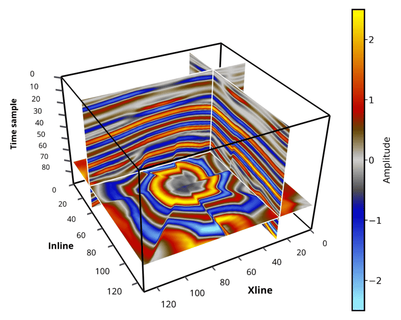
Limit slices to a useful display range

display_range restricts the visible data range along x/y/z axes. The range is also pushed into slice reads, so lazy sources do not need to load the hidden part of a slice.

This is useful for large volumes such as 600 x 500 x 1500 when the bottom time/depth samples contain mostly unused information. The bundled demo data is smaller, so we keep only the upper part of the z axis to show the workflow.

# sphinx_gallery_thumbnail_path = '_static/cigvis/3Dvispy/18.png'


import numpy as np
import cigvis
from pathlib import Path


root = Path(__file__).resolve().parent.parent.parent

sxp = root / 'data/rgt/sx.dat'
ni, nx, nt = 128, 128, 128
sx = np.memmap(sxp, np.float32, 'r', shape=(ni, nx, nt))

# Use original data coordinates and Python half-open ranges: [start, stop).
# Here x/y slices only read z samples 0..89 instead of the full 0..127 range.
display_range = {'z': (0, 90)}

nodes = cigvis.create_slices(
    sx,
    pos={'x': [36], 'y': [28], 'z': [70]},
    cmap='Petrel',
    clim=[-2.5, 2.5],
    display_range=display_range,
)
nodes += cigvis.create_axis(
    (ni, nx, display_range['z'][1] - display_range['z'][0]),
    'box',
    axis_pos='auto',
    axis_labels=['Inline', 'Xline', 'Time sample'],
)
nodes += cigvis.create_colorbar_from_nodes(nodes, 'Amplitude', select='slices')

cigvis.plot3D(
    nodes,
    view=cigvis.Plot3DView(size=(750, 600)),
    save=cigvis.Plot3DSave(path='example.png', transparent_bg=False),
)